Meta-Learning

FF15 · ©2020 Cloudera, Inc. All rights reserved

This is an applied research report by Cloudera Fast Forward Labs. We write reports about emerging technologies. Read our full report on meta-learning below or download the PDF. Our example code for applying meta-learning to an image dataset is also available.

In early spring of 2019, we researched approaches that would allow a machine learning practitioner to perform supervised learning with only a limited number of examples available during training. This search led us to a new paradigm: meta-learning, in which an algorithm not only learns from a handful of examples, but also learns to classify novel classes during model inference. We decided to focus our research report—Learning with Limited Labeled Data—on active learning for deep neural networks, but we were both intrigued and fascinated with meta-learning as an emerging capability. This report is an attempt to shed some light on the great work that’s been done in this area so far.

Introduction

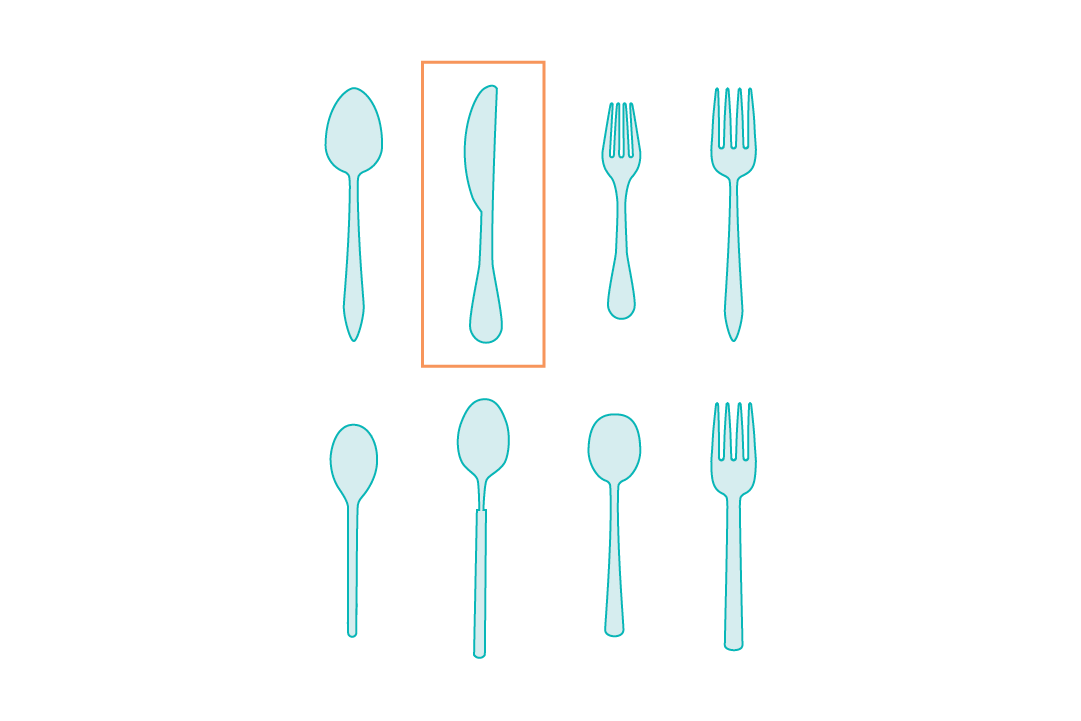
Humans have an innate ability to learn new skills quickly. For example, we can look at one instance of a knife and be able to discriminate all knives from other cutlery items, like spoons and forks. Our ability to learn new skills and adapt to new environments quickly (based on only a few experiences or demonstrations) is not just limited to identifying new objects, learning a new language, or figuring out how to use a new tool; our capabilities are much more varied. In contrast, machines—especially deep learning algorithms—typically learn quite differently. They require vast amounts of data and compute and may yet struggle to generalize. The reason humans are successful in adapting and learning quickly is that they leverage knowledge acquired from prior experience to solve novel tasks. In a similar fashion, meta-learning leverages previous knowledge acquired from data to solve novel tasks quickly and more efficiently.

Why should we care?

An experienced ML practitioner might wonder: isn’t this covered by recent (and much-accoladed) advances in transfer learning? Well, no. Not exactly. First, supervised learning through deep learning methods requires massive amounts of labeled training data. These datasets are expensive to create, especially when one needs to involve a domain expert. While pre-training is beneficial, these approaches become less effective for domain-specific problems, which still require large amounts of task-specific labeled data to achieve good performance.

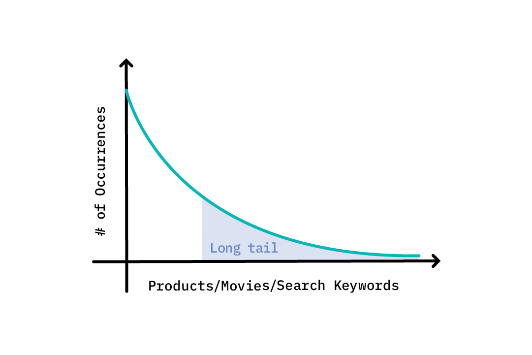
In addition, certain real world problems have long-tailed and imbalanced data distributions, which may make it difficult to collect training examples.^[1] For instance, in the case of search engines, perhaps a few keywords are commonly searched for, whereas a vast majority of keywords are rarely searched for. This may result in poor performance of models/applications based on long-tailed or imbalanced data distributions. The same could be true of recommendation engines; when there are not enough user reviews or ratings for obscure movies or products, it can hinder model performance.

Most important, the ability to learn new tasks quickly during model inference is something that conventional machine learning approaches do not attempt. This is what makes meta-learning particularly attractive.

Why now?

From a deep learning perspective, meta-learning is particularly exciting and adoptable for three reasons: the ability to learn from a handful of examples, learning or adapting to novel tasks quickly, and the capability to build more generalizable systems. These are also some of the reasons why meta-learning is successful in applications that require data-efficient approaches; for example, robots are tasked with learning new skills in the real world, and are often faced with new environments.

Further, computer vision is one of the major areas in which meta-learning techniques have been explored to solve few-shot learning problems—including classification, object detection and segmentation, landmark prediction, video synthesis, and others.^[2] Additionally, meta-learning has been popular in language modeling tasks, like filling in missing words^[3] and machine translation^[4], and is also being applied to speech recognition tasks, like cross-accent adaptation.^[5]

As with any other machine learning capability that starts to show promise, there are now libraries and tooling that make meta-learning more accessible. Although not entirely production-ready, libraries like torch-meta, learn2learn and meta-datasets help handle data, simplify processes when used with popular deep learning frameworks, and help document and benchmark performance on datasets.

The rest of this report, along with its accompanying code, explores meta-learning, provides insight into how it works, and discusses its implications. We’ll do this using a simple, yet elegant algorithm—Model Agnostic Meta-Learning^[6]—applied to a few-shot classification problem which was proposed a while ago, but continues to provide a good basis for extension and modification even today.

Framing the problem

What kind of problems can meta-learning help us solve? One of the most popular categories is few-shot learning. In a few-shot learning scenario, we have only a limited number of examples on which to perform supervised learning, and it is important to learn effectively from them. The ability to do so could help relieve the data-gathering burden (which at times may not even be possible).

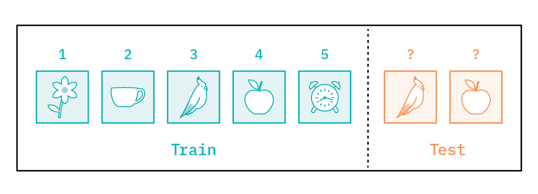
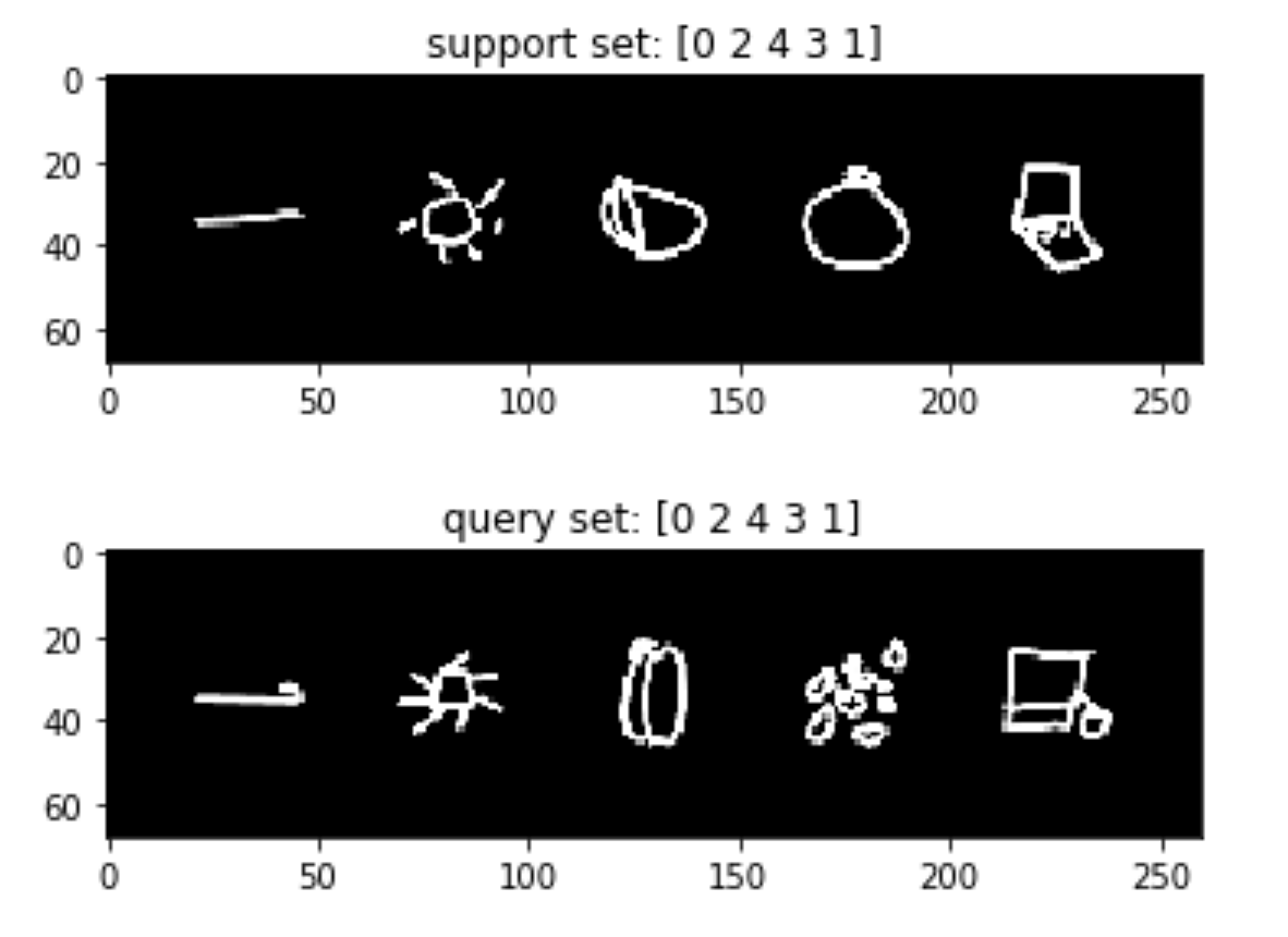
Let’s say we want to solve a few-shot classification problem, shown below in Figure 4. Usually the few-shot classification problem is set up as a N-way k-shot problem, where N is the number of classes and k is the number of examples in each class. For example, let’s say we are given an image from each of five different classes (that is, N=5 and k=1) and we are supposed to classify new images as belonging to one of these classes. What can we do? How would one normally model this?

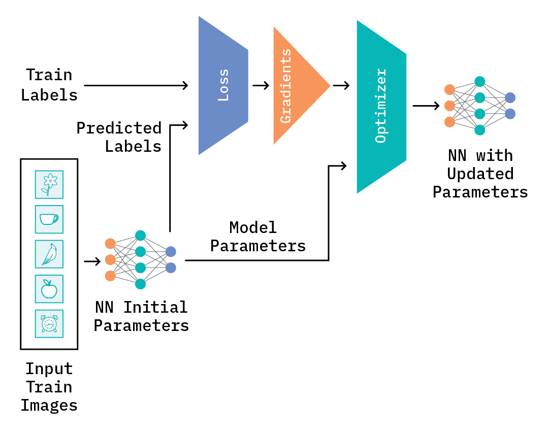
One way to solve the problem would be to train a neural network model from scratch on the five training images. At a high level, a training step will look something like Figure 5, below. The neural network model is randomly initialized and receives an image (or images) as input. It then predicts the output label(s) based on the initial model parameters. The difference between the true label(s) and the predicted label(s) is measured by a loss function (for example, cross-entropy), which in turn is used to compute the gradients. The gradients are then used to help calculate new model parameters that best reduce the difference between the “true” and predicted labels. This entire step is known as backpropagation. After backpropagation, the optimizer updates the model parameters for the model, and all of these steps are repeated for the rest of the images and/or for some number of epochs, until the loss, evaluated on the train or test data, falls below an acceptable level.

With only five images available for training, chances are that the model would likely overfit and perform poorly on the test images. Adding some regularization or data augmentation may alleviate this problem to some extent, but it will not necessarily solve it. The very nature of a few-shot problem makes it hard to solve, as there is no prior knowledge of the tasks.

Another possible way to solve the problem could be to use a pre-trained network from another task, and then fine-tune it on the five training images. However, depending on the problem, this may not always be feasible, especially if the task the network was trained on differs substantially.

Solving the problem

Data set-up

What meta-learning proposes is to use an end-to-end deep learning algorithm that can learn a representation better suited for few-shot learning. It is similar to the pre-trained network approach, except that it learns an initialization that serves as a good starting point for the handful of training data points. In the few-shot classification problem discussed, we could leverage training data that’s available from other image classes; for instance, we could look at the training data available and use images from classes like mushrooms, dogs, eyewear, etc. The model could then build up prior knowledge such that, at inference time, it can quickly acquire task-specific knowledge with only a handful of training examples. This way, the model first learns parameters from a training dataset that consists of images from other classes, and then uses those parameters as prior knowledge to tune them further, based on the limited training set (in this case, the one with five training examples).

Now the question is, how can the model learn a good initial set of parameters which can then be easily adapted to the downstream tasks? The answer lies in a simple training principle, which was initially proposed by Vinyals et. al.^[7]:

The idea is to train a model by showing it only a few examples per class, and then test it against examples from the same classes that have been held out from the original dataset, much the way it will be tested when presented with only a few training examples from novel classes. Each training example, in this case, is comprised of pairs of train and test data points, called an episode.

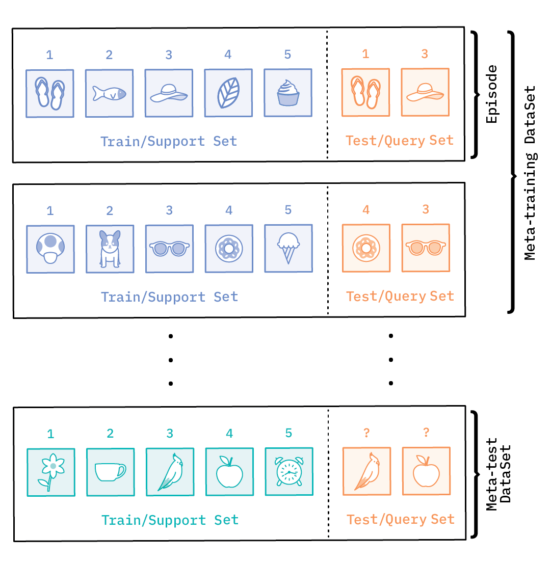
This is a departure from the way that data is set up for conventional supervised learning. The training data (also called the meta-training data) is composed of train and test examples, alternately referred to as the support and query set.

In this case, we have a 5-way, 1-shot learning problem.

Similar to conventional supervised learning, which sets aside validation and test datasets for hyper-parameter tuning and generalization, meta-learning also has meta-validation and meta-test sets. These are organized in a similar fashion as the meta-training dataset in episodes, each with support and query sets; the only difference is that the class categories are split into meta-training, validation, and test datasets, such that the classes do not overlap.

Meta-learning: learning to learn

A meta-learning model should be trained on a variety of tasks, and then optimized further for novel tasks. A task, in this case, is basically a supervised learning problem (like image classification or regression). The idea is to extract prior information from a set of tasks that allows efficient learning on new tasks. For our image classification problem, the ideal set-up would include many classes, with at least a few examples for each. These can then be used as a meta-training set to extract prior information, such that when a new task (like the one in the Figure 4, above) comes in, the model can perform it more efficiently.

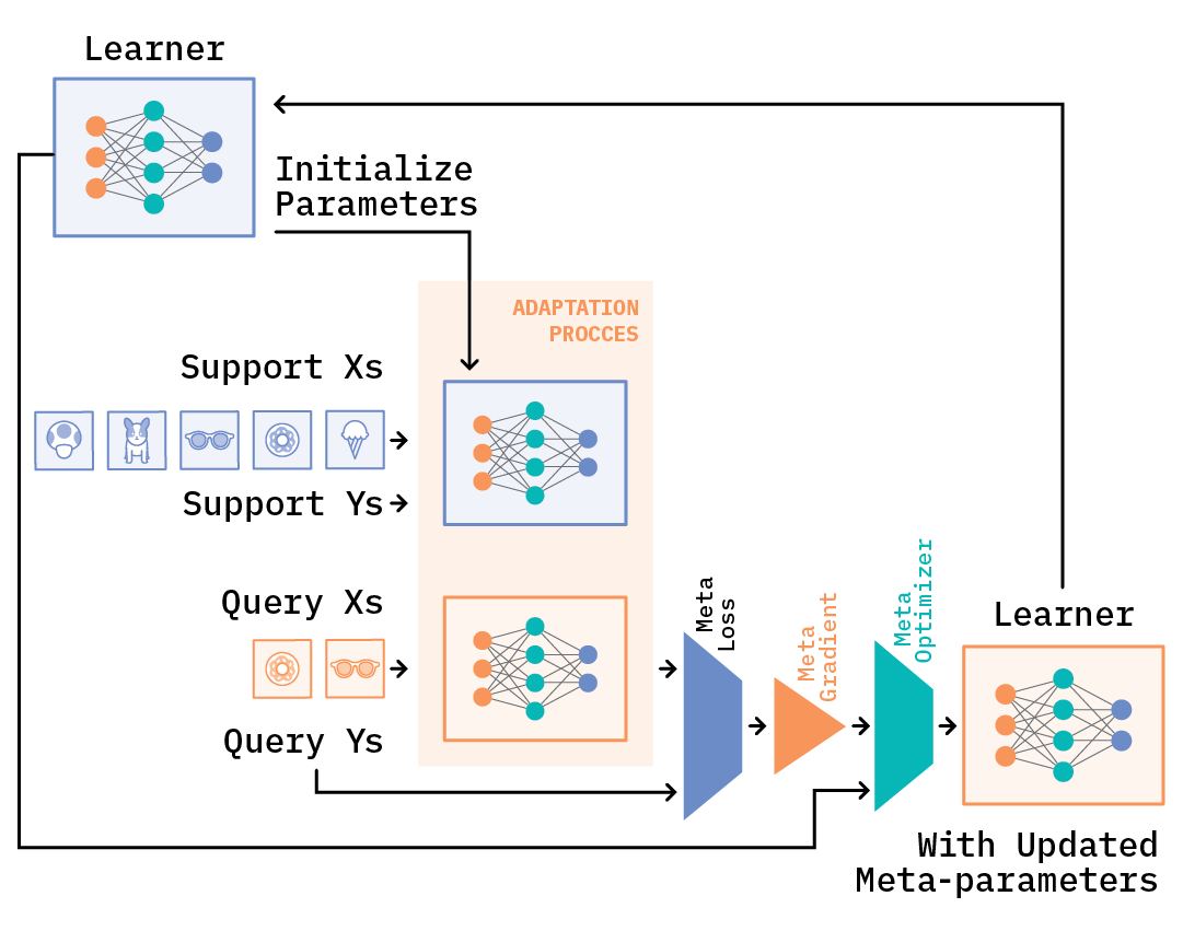
At a high level, the meta-learning process has two phases: meta-learning and adaptation. In the meta-learning phase, the model learns an initial set of parameters slowly across tasks; during the adaptation phase, it focuses on quick acquisition of knowledge to learn task-specific parameters. Since the learning happens at two levels, meta-learning is also known as learning to learn.^[8]

A variety of approaches have been proposed that vary based on how the adaptation portion of the training process is performed. These can broadly be classified into three categories: “black-box” or model-based, metric-based, and optimization-based approaches.

“Black-box” (or model-based) approaches simply train an entire neural network, given some training examples in the support set and an initial set of meta-parameters, and then make predictions on the query set. They approach the problem as supervised learning, although there are approaches that try to eliminate the need to learn an entire network.^[9]

Metric-based approaches usually employ non-parametric techniques (for example, k-nearest neighbors) for learning. The core idea is to learn a feature representation (e.g., learning an embedding network that transforms raw inputs into a representation which allows similarity comparison between the support set and the query set). Thus, performance depends on the chosen similarity metric (like cosine similarity or euclidean distance).

Finally, optimization-based approaches treat the adaptation part of the process as an optimization problem. This report mainly focuses on one of the well-known approaches in this category, but before we delve into it, let’s look at how optimization-based learning actually works.

During training, we iterate over datasets of episodes. In meta-training, we start with the first episode, and the meta-learner takes the training (support) set and produces a learner (or a model) that will take as input the test (query) set and make predictions on it. The meta-learning objective is based on a loss (for example, cross-entropy) that is derived from the test or query set examples and will backpropagate through these errors. The parameters of the meta-learner (that is, meta-parameters) are then updated based on these errors to optimize the loss.^[10]

In the next step, we look at the next episode, train on the support set examples, make predictions on the query set, update meta-parameters, and repeat. In attempting to learn a meta-learner this way, we are trying to solve the problem of generalization. The examples in the test (or query) set are not part of the training—so, in a way, the meta-learner is learning to extrapolate.

Model Agnostic Meta-learning (MAML)

Now that we have a general idea of how meta-learning works, the rest of this report mainly focuses on MAML^[11], which is perhaps one of the best known optimization-based approaches. While there have been more recent extensions to it, MAML continues to serve as a foundational approach.

The goal of meta-learning is to help the model quickly adapt to or learn on a new task, based on only a few examples. In order for that to happen, the meta-learning process has to help the model learn from a large number of tasks. For example, for the image classification problem we’ve considered, the new task is the one shown in Figure 4, while the large number of tasks could be images from other classes that are utilized for building a meta-training dataset, as shown in Figure 6.

The key idea in MAML is to establish initial model parameters in the meta-training phase that maximize its performance on the new task. This is done by updating the initial model parameters with a few gradient steps on the new task. Training the model parameters in this way allows the model to learn an internal feature representation that is broadly suitable for many tasks—the intuition being that learning an initialization that is good enough, and then fine-tuning the model slightly, will produce good results.

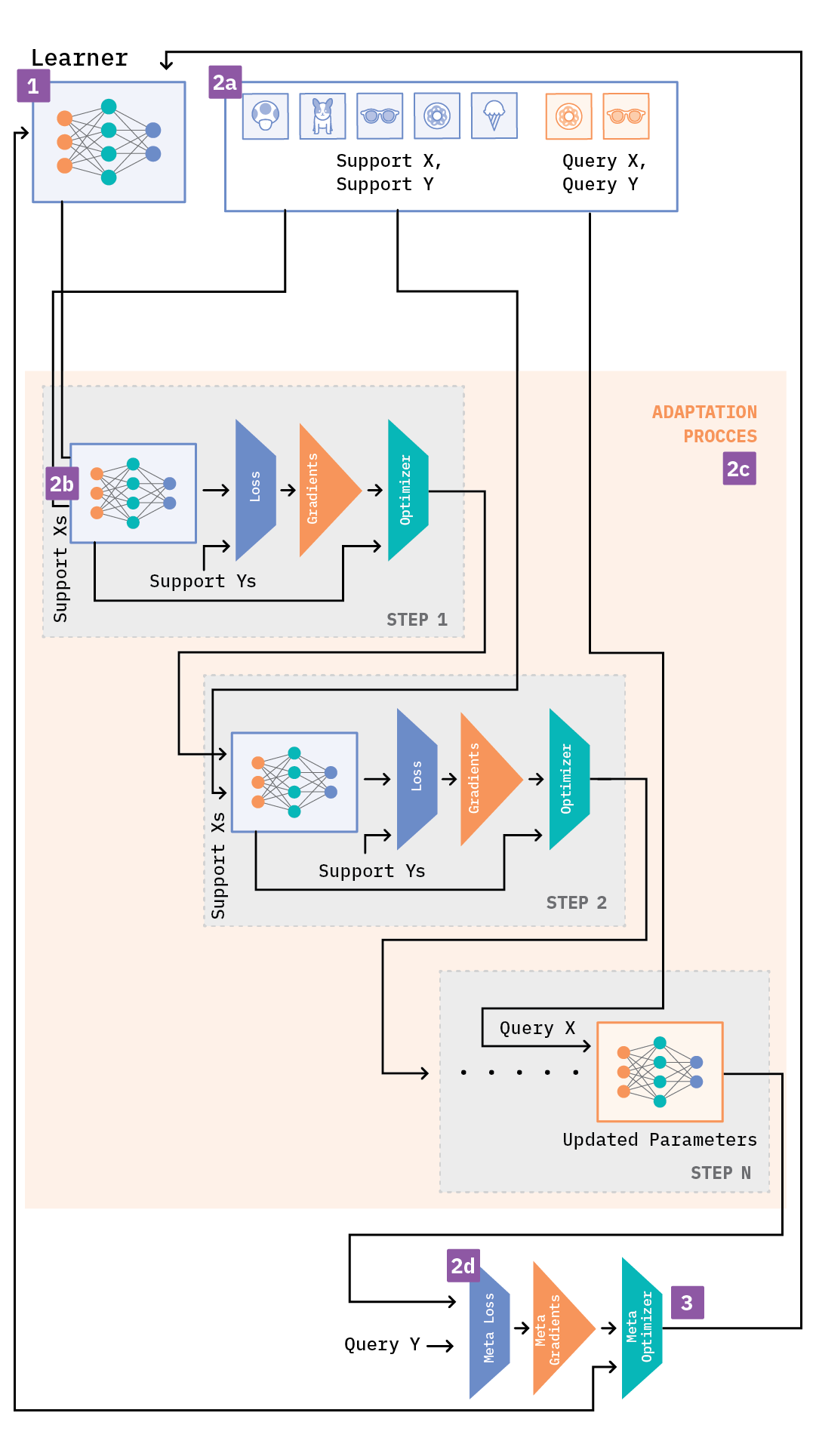
Imagine we have two neural network models that share the same model architecture:^[12] learner for the meta-learning process and adapter for the adaptation process. Since we have two models to train, we also have two different learning rates associated with them. The MAML algorithm can then be summarized in the following steps:

The “meta-loss” indicates how well the model is performing on the task. In effect, the learner is being fine-tuned using a gradient-based approach for every new task in the batch of episodes. Further, the learner acts as initialization parameters for the adapter so that it can perform task-specific learning.

During inference, we actually use the meta-trained model (learner) to predict on the meta-test set, except this time—although the meta-trained model undergoes additional gradient steps to help classify the query set examples—the learner parameters aren’t updated.

As long as the model is trained using gradient descent, the approach does not place any constraints on the model architecture or the loss function. This characteristic makes it applicable to a wide variety of problems, including regression, classification, and reinforcement learning. Further, since the approach actually undergoes a few gradient steps for a novel task, it allows the model to perform better on out-of-sample data, and hence achieves better generalization. This behavior can be attributed to the central assumption of meta-learning: that the tasks are inherently related and thus data-driven inductive bias can be leveraged to achieve better generalization.

Experiment

The MAML paper explores the approach for multiple problems: regression, classification, and reinforcement learning. To gain a better understanding of the algorithm and investigate whether MAML really learns to adapt to novel tasks, we tested the technique on the Quick, Draw! dataset. All of the experiments were performed using PyTorch (which allows for automatic differentiation of the gradient updates), along with the torch-meta library. The torch-meta library provides data loaders for few-shot learning, and extends PyTorch’s Module class to simplify the inclusion of additional parameters for different modules for meta-learning. This functionality allows one to backpropagate through an update of parameters, which is a key ingredient for gradient-based meta-learning. While torch-meta provides an excellent structure for creating reproducible benchmarks, it will be interesting to see its integration with other meta-learning approaches that handle datasets differently, and its flexibility in adopting them in the future. For our purposes, we extended the torch-meta code to accommodate the Quick, Draw! data set-up. The experiment code is available here.

Dataset

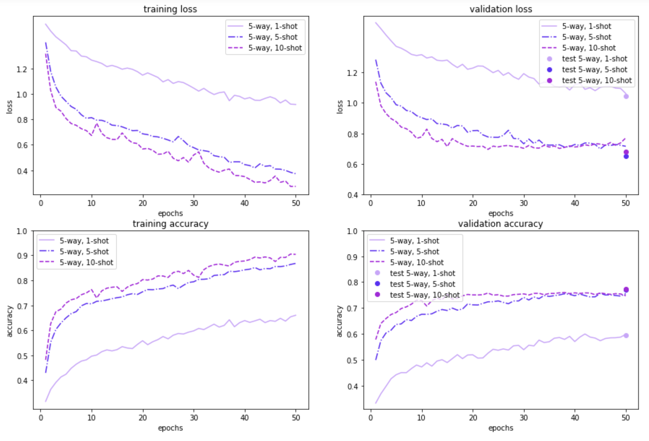
The Quick, Draw! dataset consists of 50 million doodles (hand-drawn figures) across 345 categories. We conducted two experiments: in one, we randomly selected 100 images per class; in the other, we randomly selected 20 images per class. The 345 categories were randomly split into meta-train/validation/test datasets as 207/69/69. The training and evaluation was performed on the meta-training set. The meta-validation set was mostly used for hyper-parameter tuning, and the meta-test set measured the generalization to new tasks.

Set-up

We evaluated the MAML approach on 5-way 1/5/10-shot and 10-way 1/5/10-shot settings for the Quick, Draw! dataset. An experiment on each of the 100-sample and 20-sample datasets consisted of training for 50 epochs, with each epoch consisting of 100 batches of tasks, where a task’s batch size was 25 for 100-sample and 10 for 20-sample datasets. At the end of an epoch, we evaluated the model performance on the meta-validation dataset. At the end of 50 epochs, we evaluated the model on the meta-test dataset.

In terms of model architecture, we used a network with 4 convolution layers—with size 20 channels in the intermediate representations, each including batch normalization and ReLU nonlinearities, followed by a linear layer. For all models, the loss function was the cross-entropy error between the predicted and true labels.

The models for the 100-sample dataset were trained using an SGD optimizer with a learning rate of 0.001, an inner learning rate of 0.01 for the adaptation process, a step size (that is, number of gradient steps) of 5, and a task batch size of 25. All the hyper-parameters were the same for all the models, for a consistent comparison. While the models for the 20-sample dataset were trained with a slightly lower learning rate of 0.0005, an inner learning rate of 0.005 and a task batch size of 10 while the rest of the parameters were the same as the 100-sample dataset.

Results

The figures below illustrate how MAML performs on the 100-item and 20-item randomly sampled versions of the Quick, Draw! dataset, for a 5-way or a 10-way few-shot classification problem, with a varying number of examples per class. As expected, the model performance on both the meta-validation and meta-test sets is better when the model is trained on a 100-sample subset instead of using just 20 samples. Further, 5-way classification yields better results than 10-way classification—which is to be expected, given that 5-way classification is an easier task than 10-way classification. Also, as the number of shots/examples per class increase, we see better performance during validation and test time. The validation results for 5-way 1/5/10-shot learning based on 20 samples look promising too. In the 10-way learning based on 20-samples, we see some overfitting after a few epochs, and may want to restrain the model by stopping early. That said, we have left them as is, for easy comparison with the rest of the experiment results.

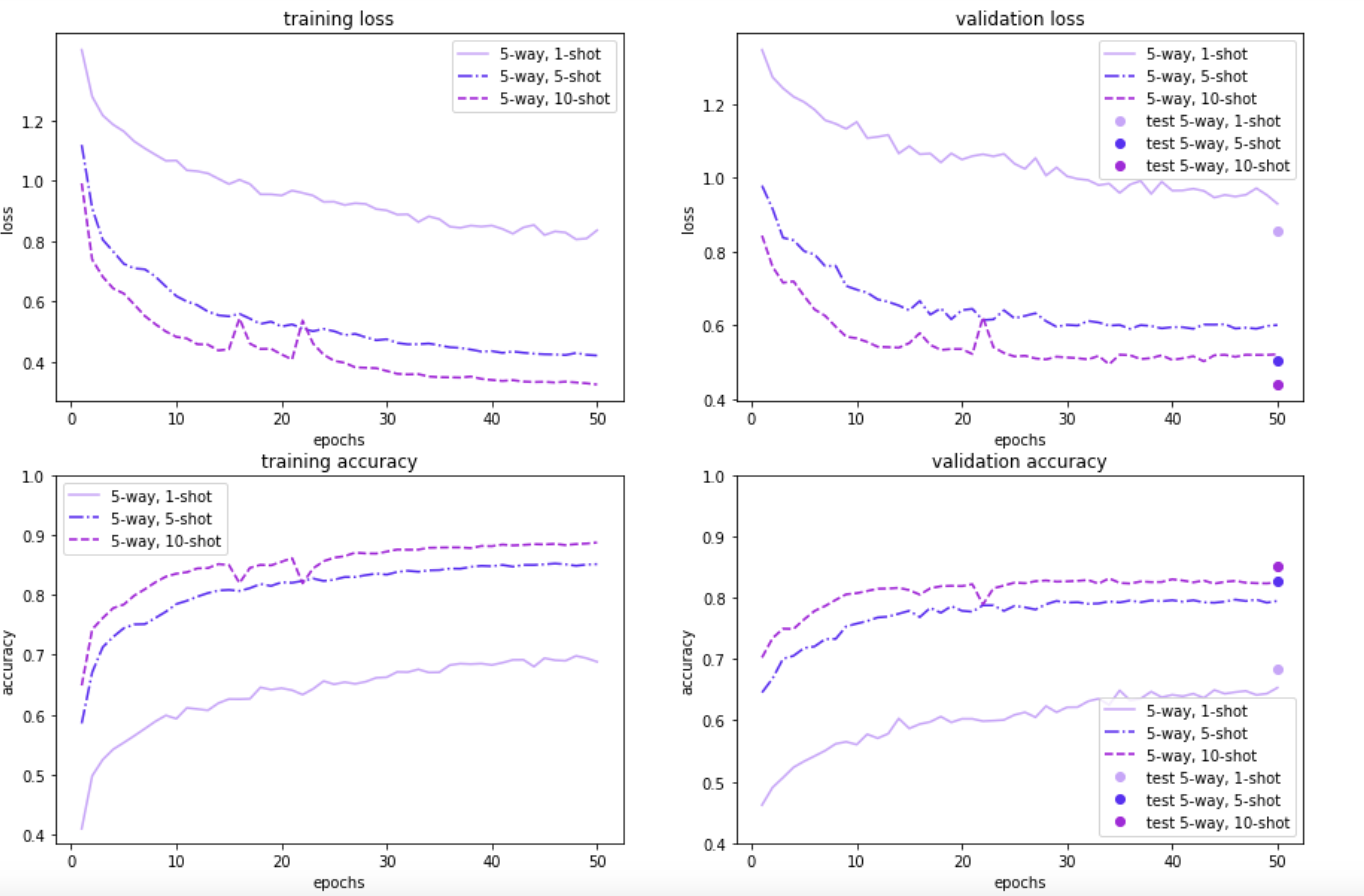
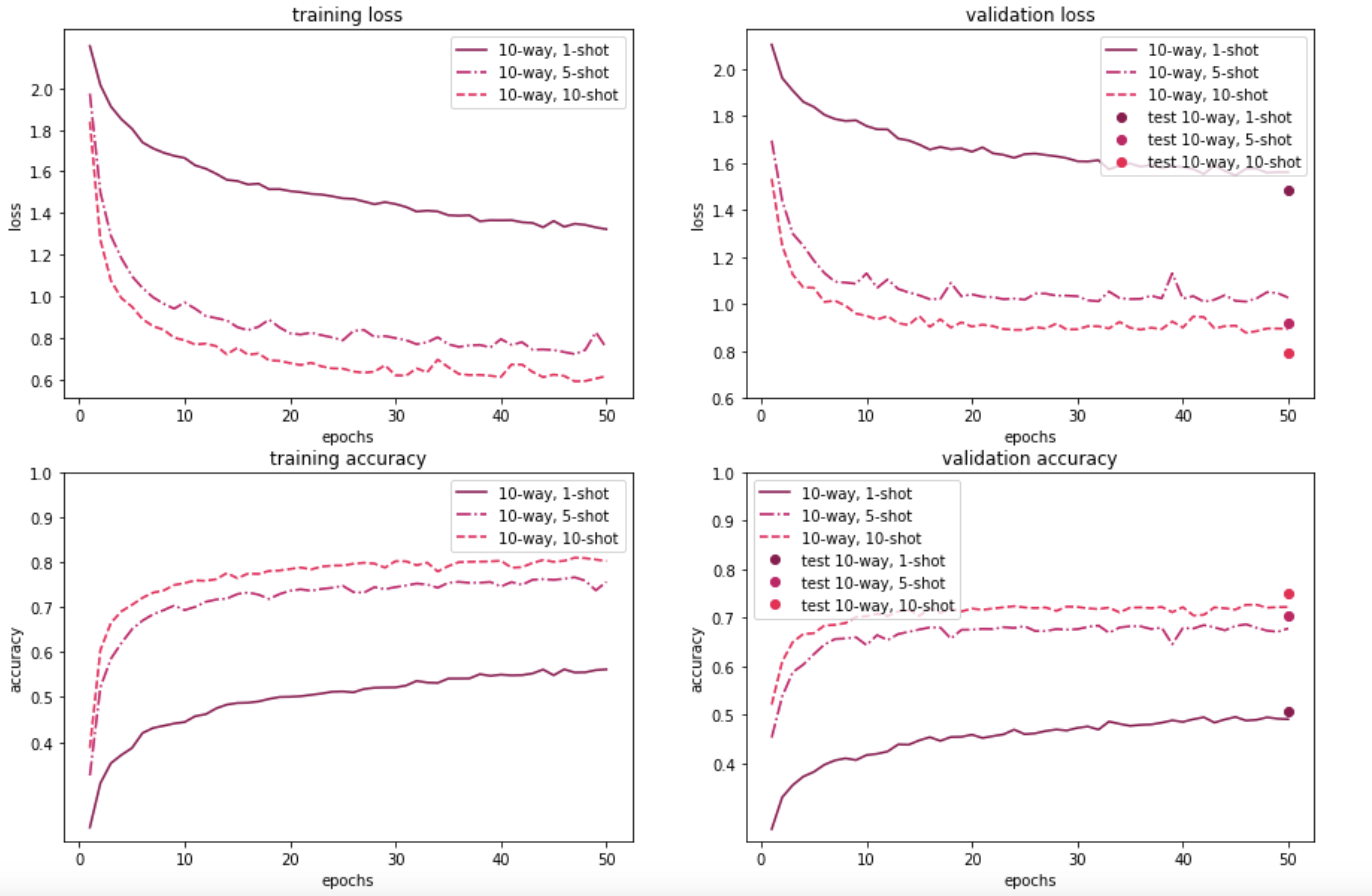
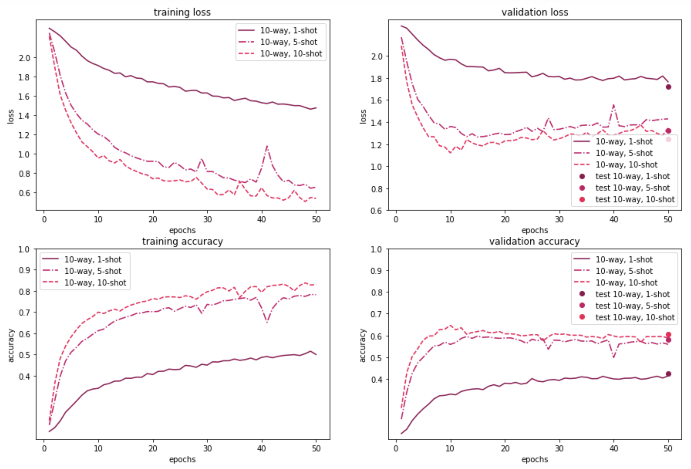
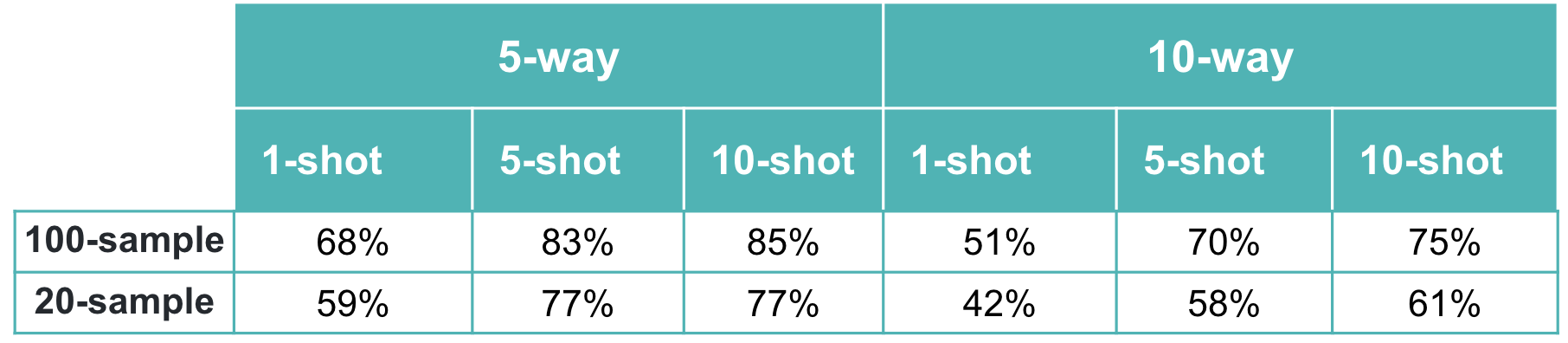
Our results demonstrate that the MAML approach is beneficial for learning with only a few examples. In the 100 randomly sampled images scenario, the 5-way classification task gives an accuracy of around 68% with just one example. The model performance is even better with additional examples; for both 5 examples and 10 examples per class, accuracy shoots over 80%. As expected, for the 10-way classification task, the results are lower (by around 10-15%), but still promising.

For the 20-random sample scenario (which is a more realistic one, from a meta-learning point of view), the 5-way results are still pretty good: ~60% accuracy with just one example. The 10-way classification results are lower, similar to the 100-sample dataset. Nonetheless, overall, the results are promising - even with minimal tuning - which suggests the applicability of the approach for fast adaptive learning.

Challenges and ways to overcome

The MAML approach fine-tunes its model using gradient descent each time for a new task. This requires it to backpropagate the meta-loss through the model’s gradients, which involves computing derivatives of derivatives, i.e., second derivatives. While the gradient descent at test time helps it extrapolate better, it does have its costs.

Backpropagating through many inner steps can be compute and memory intensive. With only a few gradient steps, it might be a less time-consuming endeavor, but it may not be the best solution for scenarios that require a higher number of gradient steps at test time. That said, the authors of the MAML paper also propose a first-order approximation that eliminates the need to compute the second derivatives, with a comparable performance. Another closely related work is OpenAI’s Reptile;^[13] it builds on first-order MAML, but doesn’t need to split the episode into support and query sets, making it a natural choice in certain settings. However, experiments suggest that approaches to reduce computation time while not sacrificing generalization performance are still in the works.^[14]

As we saw previously, learning occurs in two stages: gradual learning is performed across tasks, and rapid learning is performed within tasks. This requires two learning rates, which introduces difficulty in choosing hyper-parameters that will help achieve training stability. The two learning rates introduce hyper-parameter grid search computation - and hence, time and resources. It is also important to select the learning rate for the adaptation process carefully, because the model is learning over only a few examples. In that regard, some solutions or extensions to MAML have been developed to reduce the need for grid search or hyper-parameter tuning. For example, Alpha MAML^[15] eliminates the need to tune both the learning rates by automatically updating them as needed. MAML++, on the other hand, proposes updating the query set loss (meta-loss) for every training step in the adaptation process, which can help eliminate the training instabilities. (The authors also suggest various other steps to make it computationally efficient.)

Research that performs neural architecture search for gradient-based meta-learners^[16] also suggests that approaches like MAML and its extensions tend to perform better with deeper neural architectures for few-shot classification tasks. While note-worthy, the approach nevertheless should be explored further, with more experiments.

Ethics

Meta-learning alleviates the need to collect vast amounts of data, and is therefore applicable where supervised training examples are difficult (or even impossible) to acquire (given safety, security and privacy issues). If training efficient deep learning models is possible in such a scenario with just a handful of examples, it will benefit machine learning practitioners and meta-learning’s overall adoption.

Recent research^[17] in fairness addresses the question of how a practitioner who has access to only a few labeled examples can successfully train a fair machine learning model. The paper suggests that one can do so by extending the MAML algorithm to Fair-MAML, such that each task includes a fairness regularization term in the task losses and a fairness hyperparameter (gamma) in hopes of encouraging MAML to learn generalizable internal representations that strike a desirable balance between accuracy and fairness.

Moving forward

Meta-learning is appealing; its ability to learn from a few examples makes it particularly attractive. A gradient-based approach to meta-learning, like MAML, puts us in familiar territory: using pre-trained models and fine-tuning them. The MAML algorithm is simple, and its ability to perform a few gradient steps at inference time allows it to generalize quickly to unseen classes. The approach is applicable to a variety of problems—including regression, classification, and reinforcement learning—and can be combined with any model architecture, as long as the model is trained based on gradient descent.

While there are many areas of future research on meta-learning, here is our perspective on what could make it more adoptable in real world scenarios, as well as which areas could benefit from future work.

Some of the success of meta-learning in solving few-shot learning problems can be attributed to the way the data is set up for training and testing: episodes. In general, N-way, k-shot learning is much easier if you train the model to do N-way, k-shot learning. For our experiments, as well as the various approaches in this area, how we defined an episode was pretty arbitrary. For instance, we made an assumption that during meta-test time we would face a 5-way or a 10-way problem, with each class having either a single example or five examples. Will a real world inference scenario always match this expectation? Likely not. It could be more valuable to find an approach that can relax this assumption.

Another area worth exploring is whether it is possible to train on heterogeneous datasets. For example, can we train a meta-learning model to classify a fork based on doodles, photos of forks at restaurants, or images from product catalogs (basically, forks from different training domains or environments)? How should we define the meta-training set and episodes in such a scenario? Should we consider classes from all the environments to define the meta-train/validation/test datasets? A recent paper that applies meta-learning for few-shot land cover classification,^[18] in which the class images vary by regions (urban areas, continents, or vegetation) suggests using classes from one environment for the support set and classes from another environment for the query set. The authors find that meta-learning (MAML, actually) can benefit Earth Sciences, especially when there is a high degree of diversity in the data.

In real world scenarios, it’s often likely that we’ll have lots of unlabeled data. In such circumstances, is it possible to employ meta-learning algorithms to leverage these unlabeled datasets? The authors of one research paper^[19] propose a solution to this by augmenting a metric-based meta-learning approach to leverage unlabeled examples. In addition to the support set and the query set, the episode includes an unlabeled set. This unlabeled set may or may not contain examples from the support set classes. The idea is to use the labeled examples from the support set and the unlabeled examples within each episode to generalize for a good performance on the corresponding query set. Experiments show an improvement in model performance in some cases.

Another interesting idea that’s being explored is at the crossroads of active learning^[20] and meta-learning. The field of active learning takes advantage of machine learning in collaboration with humans, selecting examples from vast pools of unlabeled data and requesting labels for them. At times, these examples are chosen based on how uncertain the model is about its predicted label, or by how “different” it is than the rest, etc.—with the ultimate aim to improve model performance. Since there are fewer labeled training examples to begin with, one could employ meta-learning approaches in such a scenario; for instance, a metric-based approach has been discussed for batch-mode active learning.^[21] (It is also possible to learn a label acquisition strategy instead.)^[22]

Over the coming years, we will see additional approaches that will make meta-learning even more adoptable in real world scenarios; whether it’s using meta-learning successfully on heterogeneous data or leveraging unlabeled data, these approaches will make learning and generalizing with fewer labeled examples possible. As previously mentioned, we will continue to see research that simplifies both the training and inference process. These advances will allow machine learning practitioners to develop even more new ways of designing machine learning systems.

Author’s note

Thank you for reading this report. This work has been deeply influenced by the work of Professor Chelsea Finn. Also, the torch-meta library, along with its demo examples, made it easier to understand and showcase meta-learning.

---

1. Learning to Model the Tail (PDF) ↩︎

2. Meta-learning in Neural Networks: A Survey ↩︎

3. Matching Networks for One-Shot Learning ↩︎

4. Meta-Learning for Low-Resource Neural Machine Translation ↩︎

5. Learning Fast Adaptation on Cross-Accented Speech Recognition ↩︎

6. Model Agnostic Meta-learning for Fast Adaptation of Deep Networks (PDF) ↩︎

7. Matching Networks for One-Shot Learning ↩︎

8. Thrun S., Pratt L. (eds). Learning to Learn. Springer, Boston, MA. 1998. ↩︎

9. One-shot Learning with Memory-Augmented Neural Networks ↩︎

10. Note that this differs from a conventional supervised learning set-up, in which the objective is based on a loss derived only from the training set, and, of course, there is no support or query set! ↩︎

11. Model Agnostic Meta-learning for Fast Adaptation of Deep Networks (PDF) ↩︎

12. While it is possible to have two duplicate models that can share parameter tensors in popular deep learning frameworks like PyTorch, libraries like torch-meta have extended the existing torch modules to allow storing additional/new parameters. ↩︎

13. On First-Order Meta-Learning Algorithms ↩︎

14. How to train your MAML ↩︎

15. Alpha MAML: Adaptive Model Agnostic Meta Learning ↩︎

16. Auto-Meta: Automated Gradient Based Meta Learner Search ↩︎

17. Fairness warnings and fair-MAML: learning fairly with minimal data ↩︎

18. Meta-learning for Few-shot Land Cover Classification ↩︎

19. Meta-learning for semi-supervised few-shot classification ↩︎

20. A Guide to Learning with Limited Labeled Data ↩︎

21. Meta-learning for Batch Mode Active Learning (PDF) ↩︎

22. Meta-Learning Transferable Active Learning Policies by Deep Reinforcement Learning ↩︎